Fit multiple fisheries and surveys • tinyAM

Different fishing gears remove different parts of a shared population. Surveys also differ in coverage and selectivity. tinyAM represents these differences with fleet-specific fishing mortality and survey-specific catchability, while retaining one population and natural-mortality surface.

This example uses SimSurvey data loosely based on 3Ps cod: three active fisheries, an offshore RV-like survey and a coastal Sentinel-gillnet-like survey. The dataset help documents their generation and separate truth tables.

Inspect the input keys

dat <- sim_cod_obs
check_tam_data(dat)
#> ✔ Input data passed validation.
#> ℹ Years 1-20; ages 1-20; fleets: 3; surveys: 2.
head(dat$catch)
#>   year age   fleet        obs          unit mean_length
#> 1    1   1 Gillnet   9.824756 thousand fish    15.93712
#> 2    1   2 Gillnet  36.313981 thousand fish    25.19779
#> 3    1   3 Gillnet 145.173733 thousand fish    34.27789
#> 4    1   4 Gillnet 347.688565 thousand fish    42.45827
#> 5    1   5 Gillnet 446.727653 thousand fish    49.76530
#> 6    1   6 Gillnet 393.766582 thousand fish    56.41095
head(dat$index)
#>      year age       obs survey samp_time          unit mean_length
#> RV.1    1   1  827.1200     RV         0 thousand fish    15.93712
#> RV.2    1   2 2459.8000     RV         0 thousand fish    25.19779
#> RV.3    1   3 3172.5867     RV         0 thousand fish    34.27789
#> RV.4    1   4 2734.5267     RV         0 thousand fish    42.45827
#> RV.5    1   5 1415.6644     RV         0 thousand fish    49.76530
#> RV.6    1   6  983.3756     RV         0 thousand fish    56.41095

Catch has a complete year–age grid within each fleet. An unavailable catch is NA; it does not imply a closure. Each index row identifies survey and samp_time. Both simulated surveys observe the population at the beginning of each modeled year (samp_time = 0): this specifies timing, not sampling effort.

F covariates belong in catch, q covariates in index, and recruitment/N/M covariates in pop_covariates. Here mean_length is the assumed-known population mean length at age in cm, not a mean calculated from selected fish.

The Sentinel-like survey samples a coastal band more densely than the RV-like survey samples offshore. Its dome-shaped selection contrasts with ascending RV selection. Both use swept-area sampling; the Sentinel-like program does not reproduce net saturation or literal fish-per-net CPUE.

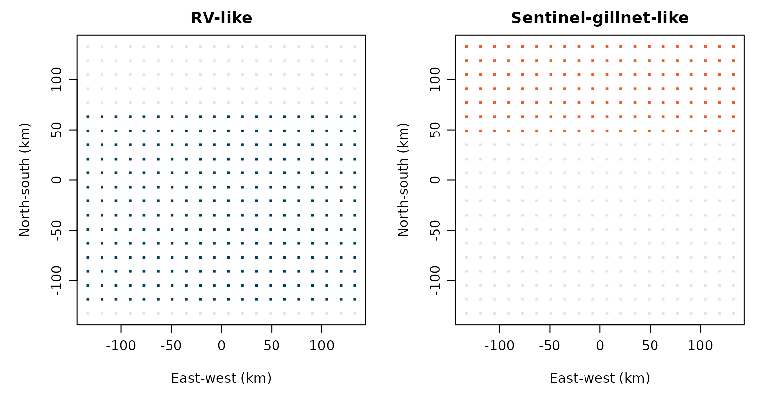
Survey footprints on the synthetic grid. The northern edge represents the coast; grey cells are outside each survey’s footprint.

Catch inputs are expanded monitoring estimates, not true catches or raw age sample counts. Genuine zeros remain in the inputs but are excluded from the lognormal likelihood. Missing biological samples are not zero catches.

This introductory scenario uses a fixed spatial pattern, a 20-by-20 grid, and log-scale SDs of 0.03 for length at age and 0.1 for total mortality, compared with 0.1 and 0.2 in the original SimSurvey paper. Static coverage keeps regional availability approximately constant; whole-fish rounding can cause small changes.

Describe each fleet within one formula

for_fleet() gives each fleet its own scale and curve. Inner formulas include intercepts, so use outer ~ 0 + to avoid an extra common baseline.

fishing <- ~ 0 +
  for_fleet("Trawl", ~ logistic(mean_length)) +
  for_fleet("Longline", ~ logistic(mean_length)) +
  for_fleet("Gillnet", ~ double_logistic(mean_length))

Trawl and longline curves ascend; the gillnet curve can decline. The generator selects individual lengths, whereas the fitted curves use mean length at age. These are approximations: a nonlinear curve at mean length need not equal mean selectivity. Realized F also reflects access, capture and depletion.

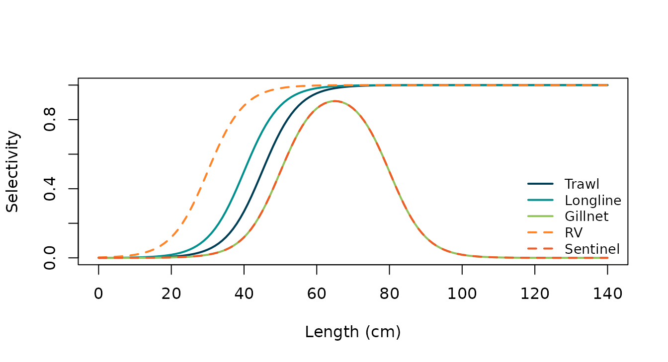
Generating selectivity curves. Dashed lines identify surveys; solid lines identify fisheries.

The raw double-logistic product is not peak-normalized; its scale is not automatically maximum F. See scopes and double-logistic help for its definition.

Give surveys their own relationships

catchability <- ~ 0 +
  for_survey("RV", ~ logistic(mean_length)) +
  for_survey("Sentinel", ~ double_logistic(mean_length))

Each survey has a separate q scale and shape. With the default log link, q is positive and can exceed one. Here it includes the fraction of the population inside the footprint. Changing regional availability would require further assumptions; it is deliberately simplified in this example.

Compare assumptions about natural mortality

The supplied M0 is a known baseline from the simulation settings, not realized M. Average it geometrically within four age blocks so that each block has one reference value per year.

breaks <- c(1, 4, 6, 11, 21)
dat$pop_covariates$M0_block <- with(dat$pop_covariates,
  exp(ave(log(M0), year, cut(age, breaks, right = FALSE), FUN = mean)))

reference_M <- fit_tam(
  dat, ages = 1:20,
  N_settings = list(process = "off", init = "exp"),
  rec_settings = list(process = "rw"),
  F_settings = list(process = "ar1", mu_form = fishing,
                   sd_form = ~ fleet, mean_ages = 5:10),
  M_settings = list(process = "off", mu_supplied = ~ M0_block,
                   age_breaks = breaks, mean_ages = 5:10),
  catch_settings = list(sd_form = ~ fleet),
  index_settings = list(q_form = catchability, sd_form = ~ survey)
)

Now allow M to vary around those same block baselines:

variable_M <- update(reference_M, M_settings = list(process = "ar1"))

check_tam(reference_M, variable_M)
#> 
#> ── reference_M ─────────────────────────────────────────────────────────────────
#> ✔ Numerical convergence: passed
#> ✔ Optimizer: 0 (relative convergence (4))
#> ✔ Max |gradient|: 0.000444 adjusted; 0.000444 raw (tolerance 0.01)
#> ✔ Positive-definite Hessian: yes
#> ✔ Model structure: no redundant model terms detected
#> 
#> Advisory findings (5):
#> ℹ 1 fixed-parameter pair(s) have absolute correlation above 0.95; inspect
#>   detailed checks.
#> ℹ Some age/series groups have mean standardized residuals outside -0.5 to 0.5.
#> ℹ Some age/series groups have standardized residual SDs outside 0.5 to 1.5;
#>   fitted-state shrinkage also affects spread.
#> ℹ Some standardized residuals exceed three SDs in absolute value.
#> ℹ Some age/series groups have absolute adjacent-year residual correlation above
#>   0.5.
#> 
#> 
#> ── variable_M ──────────────────────────────────────────────────────────────────
#> 
#> ✔ Numerical convergence: passed
#> ✔ Optimizer: 0 (relative convergence (4))
#> ✔ Max |gradient|: 0.00189 adjusted; 0.00189 raw (tolerance 0.01)
#> ✔ Positive-definite Hessian: yes
#> ✔ Model structure: no redundant model terms detected
#> 
#> Advisory findings (4):
#> ℹ Some age/series groups have mean standardized residuals outside -0.5 to 0.5.
#> ℹ Some age/series groups have standardized residual SDs outside 0.5 to 1.5;
#>   fitted-state shrinkage also affects spread.
#> ℹ Some standardized residuals exceed three SDs in absolute value.
#> ℹ Some age/series groups have absolute adjacent-year residual correlation above
#>   0.5.

The models differ only in the M process. Both use exact cohort survival, random-walk recruitment and separate AR1 F processes. M blocks share actual M; F innovations are independent between fleets, conditional on shared parameters. SD formulas distinguish fleet and survey precision. Average F/M use ages 5–10. The terminal age 20 is a plus group; the generator’s finite-age losses remain a small approximation to check.

Allowing M variation is closer to this generator than setting M equal to its baseline, but neither model is exact. Their intervals condition on known biology and baseline M; they do not establish that M is identifiable in real data. The generator partitions pre-generated total deaths, connecting fleet F and remaining M variation; the fitted fleet and M processes have separate densities.

The shared population experiences total fishing mortality,

\[ F^{\mathrm{total}}_{t,a}=\sum_f F_{t,a,f}, \qquad Z_{t,a}=M_{t,a}+F^{\mathrm{total}}_{t,a}. \]

Each fleet’s Baranov prediction uses its own F and this common Z. Catch weights determine yield; stock weights determine biomass/SSB. Catch numbers are in thousand fish and weights in kg, giving biomass in tonnes.

Inspect fleets, surveys and the common population

vis_tam(ReferenceM = reference_M, AR1M = variable_M, open_file = FALSE)

Explore the simulated-cod dashboard to inspect the example fits and diagnostics.

Start with each fleet under Fisheries, then inspect both Surveys before population trends. Aggregate fishery shows total yield without inventing aggregate standardized residuals.

ssb <- get_ssb(ReferenceM = reference_M, AR1M = variable_M)
plot_trend(ssb, color = ~model, colors = tam_pal(2), ylab = "SSB (tonnes)",
           add_buttons = FALSE) |>
  plotly::add_lines(data = sim_cod_truth$annual, x = ~year, y = ~SSB,
    inherit = FALSE, name = "Generating SSB",
    line = list(color = "#333333", dash = "dot"),
    hovertemplate = "%{x}<br>%{y} tonnes<extra>Generating SSB</extra>") |>
  add_plot_buttons()

plot_matrix(get_f(variable_M))

The dotted line is known SSB, without a confidence interval. The table measures relative error, (estimate - truth) / truth, across years and at the terminal year; mean absolute relative error prevents errors of opposing signs from canceling.

Model	Mean SSB (tonnes)	Mean RE (%)	Mean ARE (%)	Terminal RE (%)
ReferenceM	48663.9	-6.6	8.8	-13.7
AR1M	51232.6	-3.7	6.7	-13.1

These compare historical estimates with truth for one selected teaching realization, not forecast skill, simulation-study bias or coverage. Mean errors for AR1M abundance and recruitment are -21.8% and -28.9%. Agreement in SSB does not guarantee recovery of every population quantity. get_f() returns total F; fleet-specific F is in tidy_pop(variable_M)$F_fleet. Use generating truth to evaluate results, not to alter observations.

As a further hypothesis, remove age-dependent q while retaining survey scales:

flat_q <- update(variable_M, index_settings = list(q_form = ~ survey))